Help

3. Rate Calculation

3.1 Presentation
Astrophysica for Windows computes numerically resonant as well as non-resonant reaction rates. The methods used are detailed in the reference:

Nacre compilation, C. Angulo et al. , Nucl. Phys. A656 (1999) 3

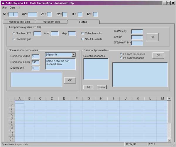
At startup, the screen looks like:

First you have to enter masses, charges, and spins (see convention for spins)
First you have to enter data by selecting a tab (Non-resonant or Resonant data). These data can also be imported from an external file (Data -> Import). The structure of the files is detailed below.
For non-resonant rates, you have first to perform polynomial fit(s), which will be used for the rate calculation.

Once the data are introduced and polynomial fits have been done (non-resonant rate), select the tab "Rate" and give the conditions of the calculation.

The standard temperature grid is the one adopted by the Caltech and NACRE compilations. The program provides the rates in a numerical form, and an analytical approximation.

3.2 Importing files

Before computing the rate you have, either to introduce data manually, or to import a data file. This file should be located on your computer or downloaded form the NACRE server. The structure of the files are detailed below.

3.3 Non-resonant rate

The structure of the S-factor file has the following structure:

A1, A2, Z1, Z2, I1, I2	One line
Ecm (in MeV), S-factor (in MeV-barn), Error on S (optional, in MeV-barn)	(repeat for each energy)

The numbers must be separated by blanks with coma's. A fourth input can be given to give a label to the data set.

Example:

4 3 2 1 0 1
0.18  1.2e-5 1.3e-6 GR62 
0.39  3.13e-4 1.11e-5
0.64  5.7e-4 1.1e-4 WA63 
1.47  0.000015  0.0000024
1.58  0.000016  0.0000018
3.49  0.000045  0.0000016 BE64 
4.49  0.00006  0.0000022
5.48  0.00007  0.0000029

The labels GR62, WA63 and BE64 are used to distinguish between different data sets.

Required input:

Temperature range.
Number of points (standard value=100): used for the numerical integration of the cross section times the Maxwell distribution.
Number of widths (standard value= 3): the integration range goes from E0-nwidths*DE0 to E0+nwidths*DE0.
Npol (standard value= 3): degree of the polynomial fit.

3.4 Example of non-resonant rate

We take the t(a,g)⁷Li reaction as an example. The data file tag.nr is provided with the package. Follow the procedure:

Introduce the masses, charges and spins of triton and alpha.
Menu Data -> import -> Non-resonant file. Open tag.nr. Four data sets are given in a tabular form on the left, and on a graphical form on the right.
Perform polynomial fits (order 2 and 3 for example).
Select the tab "Rates" on the top of the window.
Select "Standard grid" in the temperature grid. Try "Give Caltech data" and/or "Give Nacre data".
Select one the polynomial fits performed before (step 3). You can also choose a linear interpolation between the data points.
Click "OK" in the "Non-resonant parameters" panel.

When choosing degree 2 for the S-factor fit, you get the following results.

The analytical approximation reads:

5.93E05 /T23*exp(- 8.072/T13)*(1-9.545E-02*T^1+3.894E-02 *T^2-9.408E-04*T^3)

3.5 Resonant reaction rate

Resonance properties must be given, either manually by filling up the "Resonant data" tab, or by importing a file from your computer.
Data are:

l (column A): orbital angular momentum.
J (column B): total spin of the resonance.
E (column C): c.m. energy (negative for subthreshold states, in MeV).
Gp (column D): particle width in the entrance channel (in MeV).
If E<0, Gp is the reduced width (in MeV).
Gg (column E): gamma width in the entrance channel (in MeV)
Gtot (column F): total particle width (in MeV).
In general, Gp=Gtot, but it can different if several particle channels are open. Example: ¹⁰B(p,g)¹¹C.
a (column G): radius (in fm).
Ef (column H): Final state energy (in MeV) with respect to the threshold (always negative! ).
lam (column I): Order of the multipole.

Important remark: the full set of data enables you to compute the resonant contribution, including the tail contribution. If Gp is <0, Gp is the resonance strength wg, and the tail contribution is neglected. In this case, columns E to I are not used

Then in the "Rates" tab, temperature range must be given (see above).
You may select a part of the resonance set, and then compute the rate. The fit can be performed, either on each resonance individually, or within a multiresonance approximation.

3.6 Example of resonant reaction rate

The ²³Na(p,g)²⁴Mg reaction is taken as an example. The input file is given below:

 22.9878  1.0078 11  1  3  1                                                
  0  2 -1.170E-01  1.600E-07  1.000E-01   1.000E-01 4.610E+00 -1.169E+01  2
  0  2  2.420E-01  8.040E-10  2.000E-05   2.000E-05 4.610E+00 -1.169E+01  2  
  0  2  2.760E-01  4.000E-10  1.800E-03   1.800E-03 4.610E+00 -1.169E+01  2   
  0  2  2.980E-01  1.680E-07  2.000E-06   2.000E-06 4.610E+00 -1.169E+01  2   
  0  0  3.270E-01 -6.250E-10   .000E+00    .000E+00  .000E+00   .000E+00  0   
  0  0  3.610E-01 -1.380E-09   .000E+00    .000E+00  .000E+00   .000E+00  0   
  0  0  4.300E-01 -6.250E-10   .000E+00    .000E+00  .000E+00   .000E+00  0

The first state corresponds to a subtreshold state. For states 5, 6 and 7, only wg is introduced. The resulting file is available here.